Facts about Classification

📌 Need for Cross-Validation

✅ Why is Cross-Validation Needed?

In any machine learning model, if the model performs poorly on the test data, we typically adjust the hyperparameters or switch to a different model. If we repeat this process multiple times, there is a chance that we might achieve good accuracy on the test data without overfitting. However, despite this, the model might still perform poorly on unseen data. The reason for this is that we measured the generalization error multiple times on the test set, causing the model and its hyperparameters to adapt specifically to that set. As a result, the model becomes overly optimized for the test set and is unlikely to perform well on new, unseen data.
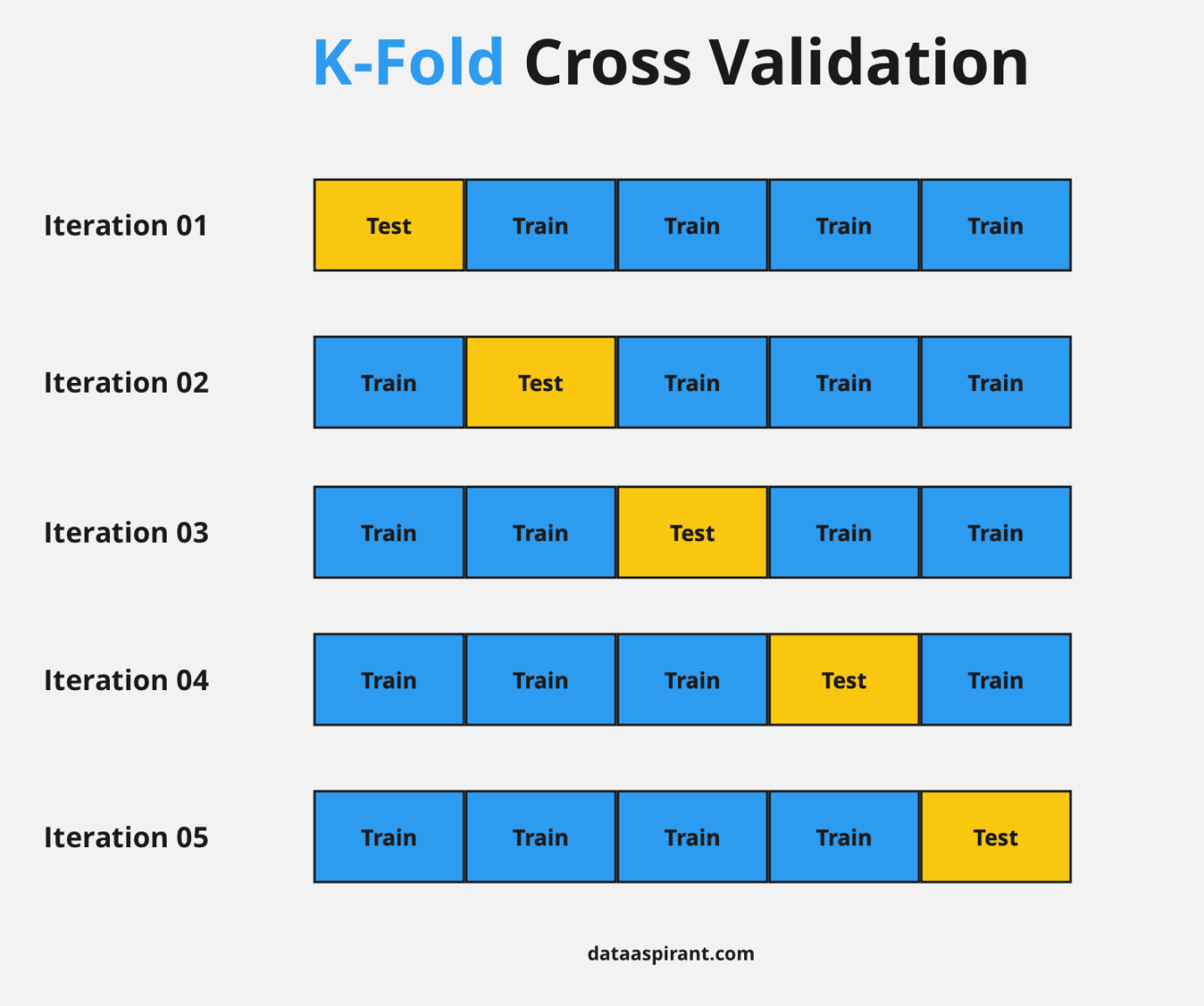
Cross Validation

Figure: K-Fold Cross Validation

    Benefits:
                            
  • Ensures the model performs well on unseen data by validating its performance across multiple subsets, reducing the risk of overfitting.
  • Provides a more reliable evaluation by using all data for both training and validation, reducing variance in performance metrics.
  • Ensures every data point is used for both training and validation, maximizing the utility of the dataset.
  • Helps identify the best model configuration by evaluating performance across different hyperparameter settings.

Pseudo-Example of K-Fold Cross-Validation

    Dataset = [D1, D2, D3, D4, D5]
    K = 5  # 5-Fold Cross Validation

    Iteration 1: Train on [D2, D3, D4, D5], Test on [D1]
    Iteration 2: Train on [D1, D3, D4, D5], Test on [D2]
    Iteration 3: Train on [D1, D2, D4, D5], Test on [D3]
    Iteration 4: Train on [D1, D2, D3, D5], Test on [D4]
    Iteration 5: Train on [D1, D2, D3, D4], Test on [D5]

    Final Model Performance = Average of all 5 test results
        

🚀 Key Takeaways

  • K-Fold Cross Validation ensures **each data point** is tested once.
  • More folds (e.g., K=10) provide a **smoother estimate** of accuracy.
  • Cross-validation is **crucial for small datasets** where a single split may be misleading.

What is k-fold cross validation?

By reducing the training data, we risk losing important patterns/trends in the data set, which in turn increases error induced by bias. With k-fold CV, we will have enough data for training & validation.

After splitting the total data set (Dn) into training (DTrain) and test (DTest) data sets in the ratio of 80:20, we further randomly split the training data into k equal parts. E.g.:

We have to randomly split the data set into k equal parts, then compute k different accuracies for each hyperparameter value and take their mean. Time complexity for k folds will be k * n * d, making it O(knd), where k is the number of folds.

Generally, k = 5, 10 is preferred.

Example of 5-Fold Cross Validation:

In a **5-Fold Cross Validation**, the training data is split into **5 equal parts**. In each iteration:

This process is repeated **5 times**, with each fold being the test set once.

Formula for Final Performance Score:

The final performance is calculated as the **mean of the individual performances** across all k iterations:
Performance = (1/k) * Σ Performancei for i=1 to k

Time Complexity of K-Fold Cross Validation

We must compute k different accuracies for each hyperparameter value and take their mean. The time complexity for k folds is **O(k * n * d)**, where:

Generally, **k = 5 or 10** is preferred.

What is KD-Tree?

A K-Dimensional Tree (KD-Tree) is a binary tree used for organizing points in k-dimensional space. It is mainly used for nearest neighbor search, range queries, and spatial indexing.

Example: Constructing a KD-Tree

Let's consider a set of 2D points: (7,2), (5,4), (9,6), (2,3), (4,7), (8,1).

  1. Step 1: Choose the first axis (x-axis) and sort points by x-coordinate.
  2. Step 2: Select the median point as the root. Here, (7,2) is the root.
  3. Step 3: Recursively split the remaining points using alternating axes (x → y → x...).

Time Complexity of KD-Tree

  • Build Time Complexity: O(n log n)
  • Nearest Neighbor Search (Best Case): O(log n)
  • Nearest Neighbor Search (Worst Case): O(n) (if the tree is unbalanced)

How KD-Tree Helps in KNN?

When searching for the nearest neighbors of a query point, the KD-Tree:

  • Prunes irrelevant branches of the tree.
  • Reduces the number of distance calculations.
  • Significantly speeds up search compared to brute-force O(n) search.

Use Cases

  • Image Recognition (e.g., finding similar images)
  • Geospatial Search (e.g., finding nearby locations on a map)
  • Machine Learning (e.g., used in KNN for fast classification)

The diagram above illustrates how a KD-Tree partitions the space step by step. Each split divides the space based on an alternating axis (x, then y, then x again, etc.).

What is Locality Sensitive Hashing (LSH)?

Locality Sensitive Hashing (LSH) is a technique used for approximate nearest neighbor search in high-dimensional spaces. Unlike traditional hashing methods, LSH increases the probability that similar data points will be mapped to the same hash bucket. This makes LSH useful in applications such as document similarity, image retrieval, and recommendation systems.

Example of LSH:

Suppose we have the following three text documents:

  • Doc 1: "The quick brown fox jumps over the lazy dog"
  • Doc 2: "The fast brown fox leaps over the sleepy dog"
  • Doc 3: "A red apple is on the table"

Using LSH with a MinHash function for text similarity, Doc 1 and Doc 2 would likely hash to the same bucket because they contain similar words. However, Doc 3 is quite different and would hash to a different bucket.

How It Works:

  1. Convert documents into sets of words (or shingles).
  2. Compute MinHash signatures for each document.
  3. Use multiple hash functions to group similar documents into the same bucket.
  4. Retrieve similar documents by checking within the same bucket.

Benefits of LSH:

  • Efficient for high-dimensional data
  • Speeds up nearest neighbor searches
  • Used in search engines, plagiarism detection, and machine learning applications

What is the Curse of Dimensionality?

The Curse of Dimensionality refers to the various problems that arise when working with high-dimensional data. As the number of dimensions increases, the volume of the space grows exponentially, leading to sparsity and increased computational complexity. This phenomenon can cause issues such as overfitting, increased distance between data points, and the need for more data to maintain statistical significance.

Effects of the Curse of Dimensionality:

  • Increased computational complexity
  • Sparsity of data points
  • Increased distance between data points
  • Overfitting due to the abundance of features
  • Need for more data to maintain statistical significance

Strategies to Mitigate the Curse of Dimensionality:

  • Feature selection and dimensionality reduction techniques
  • Regularization to prevent overfitting
  • Use of domain knowledge to reduce irrelevant features
  • Feature engineering to create meaningful features
  • Model selection based on the complexity of the data

Reachability Distance & Local Reachability Density

Reachability Distance:

Reachability distance expresses the maximum of the distance between two points and the k-distance of the second point. The distance metric used can be Euclidean, Minkowski, Manhattan, or any other distance measure.

Formula:

Reachability_Distance(a, b) = max{ k-distance(b), normal_distance(a, b) }

Local Reachability Density:

Local reachability density refers to how far we need to go from a given point to reach its neighboring points. The reachability distances of the k closest neighbors of a point are used to calculate the local reachability density. The sum of these reachability distances is divided by k, and the inverse of this value gives the desired density.

Formula:

Local_reachability_density(a) = 1 / ( sum( Reachability_Distance(a, n) ) / k )

Where n refers to the k nearest neighbors of point a.

Local Outlier Factor (LOF)

The Local Outlier Factor (LOF) is a measure used to identify the degree to which a data point deviates from its neighbors. It is based on the concept of local density and is particularly useful for detecting outliers in datasets with varying densities.

How LOF Works:

  • LOF compares the local reachability density of a point with those of its k-nearest neighbors.
  • If a point has a significantly lower local reachability density than its neighbors, it is considered an outlier.
  • LOF values greater than 1 indicate outliers, where higher values signify stronger anomalies.

Formula:

LOF(a) = ( sum( Local_reachability_density(n) / Local_reachability_density(a) ) ) / k

Where n refers to the k-nearest neighbors of point a.

Interpretation:

  • LOF ≈ 1 → The point is in a dense region (normal).
  • LOF > 1 → The point is in a sparse region (potential outlier).
  • Higher LOF → Stronger outlier indication.