Understanding K-Nearest Neighbors (KNN)

K-Nearest Neighbors (KNN) is a simple, yet powerful, supervised learning algorithm used for classification and regression. It makes predictions based on the majority class of its nearest neighbors.

Steps to Calculate KNN

1. Choose the Number of Neighbors (K)

The first step is to select the number of neighbors (K). A small K value (e.g., K=3) makes the model more sensitive to noise, while a larger K value provides smoother decision boundaries.

2. Compute the Distance

For a given query point, calculate the distance between it and all other points in the dataset. The most common distance metric is the Euclidean distance, which is computed as:

Euclidean Distance Formula:
d=√((x₂ - x₁)² + (y₂ - y₁)²) 

3. Identify the K Nearest Neighbors

Sort all the distances in ascending order and select the top K closest points to the query point.

4. Determine the Majority Class

Among the K nearest neighbors, count the occurrences of each class label. The class with the highest count is assigned to the query point.

5. Assign the Class to the Query Point

The final step is to classify the query point based on the majority class of its nearest neighbors.

Example: Toy Dataset

Let's consider a small dataset where we have points classified into two categories (0 and 1).

X	Y	Label
1	2	0
2	3	0
3	3	0
6	8	1
7	8	1
8	7	1

Now, if we have a query point at (5, 5) and choose K=3, we calculate distances:

Point (X, Y)	Distance to (5, 5)	Label
(1, 2)	5.00	0
(2, 3)	3.61	0
(3, 3)	2.83	0
(6, 8)	3.16	1
(7, 8)	3.61	1
(8, 7)	3.61	1

The 3 nearest neighbors are:

(3, 3) - Class 0
(6, 8) - Class 1
(2, 3) - Class 0

Since Class 0 appears twice and Class 1 appears once, the query point (5, 5) is classified as Class 0.

Key Characteristics of KNN

KNN is a non-parametricalgorithm, meaning it makes no assumptions about the data distribution.
It is a lazy learner, meaning it stores the training data and makes predictions at runtime.
It works well with small datasets but can become slow for large datasets due to distance calculations.

Conclusion

KNN is an intuitive and effective algorithm for classification tasks. However, choosing an optimal K value and handling large datasets efficiently are key challenges in using KNN.

Failure Cases of KNN

1. High Computational Cost

KNN stores all training data and computes distances at runtime, making it slow for large datasets.

2. Curse of Dimensionality

As the number of features increases, distance calculations become less meaningful, reducing accuracy.

3. Sensitive to Noisy Data

KNN is easily affected by outliers and mislabeled data, which can lead to incorrect classifications.

4. Imbalanced Data Problem

If one class is much larger than the others, KNN may be biased toward the majority class.

5. Choosing the Wrong K Value

Too small a K value makes KNN sensitive to noise, while too large a K value may cause misclassification.

Distance Measures in Machine Learning

1. Euclidean Distance (L2 Norm)

It represents the straight-line distance between two points.

Formula: d(A, B) = √(∑ (Aᵢ - Bᵢ)²)

Example: Given two points A(2, 3) and B(5, 7):

d(A, B) = √((5 - 2)² + (7 - 3)²) = √(9 + 16) = √25 = 5

2. Manhattan Distance (L1 Norm, City Block Distance)

Measures the sum of absolute differences between coordinates.

Formula: d(A, B) = ∑ |Aᵢ - Bᵢ|

Example: Given two points A(2, 3) and B(5, 7):

d(A, B) = |5 - 2| + |7 - 3| = 3 + 4 = 7

3. Minkowski Distance

A generalized distance metric.

Formula: d(A, B) = (∑ |Aᵢ - Bᵢ|ᵖ)^(1/p)

Example: With p=3, given A(2, 3) and B(5, 7):

d(A, B) = (|5 - 2|³ + |7 - 3|³)^(1/3) = (27 + 64)^(1/3) ≈ 4.64

4. Hamming Distance

Counts differing positions in binary or categorical data.

Formula: d(A, B) = ∑ 𝟙(Aᵢ ≠ Bᵢ)

Example: Comparing A = "1011101" and B = "1001001":

d(A, B) = Differences at 3rd, 5th, and 6th positions → Hamming Distance = 3

5. L1 Norm (Taxicab Norm)

Another name for Manhattan Distance.

Formula: ||A||₁ = ∑ |Aᵢ|

Example: A vector A = (3, -4, 5):

||A||₁ = |3| + |-4| + |5| = 3 + 4 + 5 = 12

6. L2 Norm (Euclidean Norm)

Another name for Euclidean Distance.

Formula: ||A||₂ = √(∑ Aᵢ²)

Example: A vector A = (3, -4, 5):

||A||₂ = √(3² + (-4)² + 5²) = √(9 + 16 + 25) = √50 ≈ 7.07

Summary Table:

Distance Metric	Formula	Example
Euclidean (L2)	√(∑ (Aᵢ - Bᵢ)²)	d((2,3), (5,7)) = 5
Manhattan (L1)	∑ \|Aᵢ - Bᵢ\|	d((2,3), (5,7)) = 7
Minkowski (p=3)	(∑ \|Aᵢ - Bᵢ\|³)^(1/3)	d((2,3), (5,7)) ≈ 4.64
Hamming	∑ 𝟙(Aᵢ ≠ Bᵢ)	d("1011101", "1001001") = 3
L1 Norm	∑ \|Aᵢ\|	\|\| (3, -4, 5) \|\|₁ = 12
L2 Norm	√(∑ Aᵢ²)	\|\| (3, -4, 5) \|\|₂ ≈ 7.07

Cosine Similarity & Cosine Distance

1. Cosine Similarity

Cosine similarity measures the cosine of the angle between two vectors.

Formula:

Cosine Similarity = \( \cos(\theta) = \frac{A \cdot B}{||A||_2 ||B||_2} \)

Example:

For vectors A(3,4) and B(4,3):

Dot product: \( 3 \times 4 + 4 \times 3 = 24 \)

Magnitude of A: \( \sqrt{3^2 + 4^2} = 5 \)

Magnitude of B: \( \sqrt{4^2 + 3^2} = 5 \)

Cosine Similarity: \( \frac{24}{5 \times 5} = 0.96 \) (Highly similar)

2. Cosine Distance

Cosine distance is derived from cosine similarity:

Formula:

Cosine Distance = \( 1 - \cos(\theta) \)

For our example: \( 1 - 0.96 = 0.04 \) (Very small distance)

3. Relationship with Euclidean Distance

For normalized vectors, Euclidean distance and cosine similarity are related:

\( d_{\text{Euclidean}}^2 = 2 (1 - \cos(\theta)) \)

4. Visual Representation

The diagram below illustrates the difference between Euclidean Distance and Cosine Similarity.

Cosine Similarity vs. Euclidean Distance Diagram

How Good KNN is ?

Performance of KNN for Amazon Fine Food Reviews (364K Data Points)

1. Time Complexity of KNN

Training Time: \( O(1) \) (No model training required)

Prediction Time:

Brute Force Search: \( O(N \times d) \) per query
Using KD-Tree / Ball-Tree (for low dimensions): \( O(\log N) \)
Using Approximate Nearest Neighbors (FAISS, Annoy): \( O(k \log N) \)

Issue: For \( N = 364K \), brute-force KNN is very slow.

2. Memory Complexity of KNN

Memory usage depends on the number of features \( d \).

TF-IDF (Sparse Matrix, 364K × 10K): ~3-5 GB RAM
Word2Vec (Dense Matrix, 364K × 300): ~400 MB RAM
BERT Embeddings (364K × 768): ~2.2 GB RAM

Issue: KNN stores the entire dataset in memory, making it inefficient for large datasets.

3. Performance Bottlenecks

Predicting one review takes minutes using brute-force KNN.
High RAM usage due to storing all 364K reviews.

4. Optimizations for KNN on Large Datasets

✅ Use Approximate Nearest Neighbors (ANN)
- FAISS (Facebook AI Similarity Search) - Fast and scalable.
- Annoy - Optimized for large datasets.
- HNSW - Graph-based nearest neighbors search.
✅ Dimensionality Reduction
- PCA (Reduces 300 features to ~50).
- t-SNE / UMAP for visualization.
✅ Use Faster Algorithms
- Naïve Bayes (Fast for text classification).
- SVM, Logistic Regression (More scalable).
- Transformer Models (BERT, RoBERTa - Best accuracy).

5. Conclusion: Should You Use KNN for 364K Reviews?

❌ Not recommended for real-time applications.
❌ High memory usage makes it inefficient.
✅ Works if you use optimizations (FAISS, dimensionality reduction).
✅ Use KNN only if interpretability is crucial.

Alternative: Consider SVM, Naïve Bayes, or Transformer-based models for better performance.

Decision Surface in K-Nearest Neighbors (KNN)

1. What is a Decision Surface?

A decision surface (or boundary) is the dividing line that separates different classes in a classification problem. In KNN, the shape of the decision surface depends on the number of neighbors (K).

2. How the Decision Surface Changes with K?

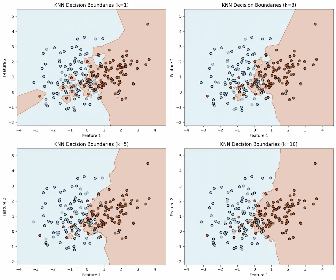
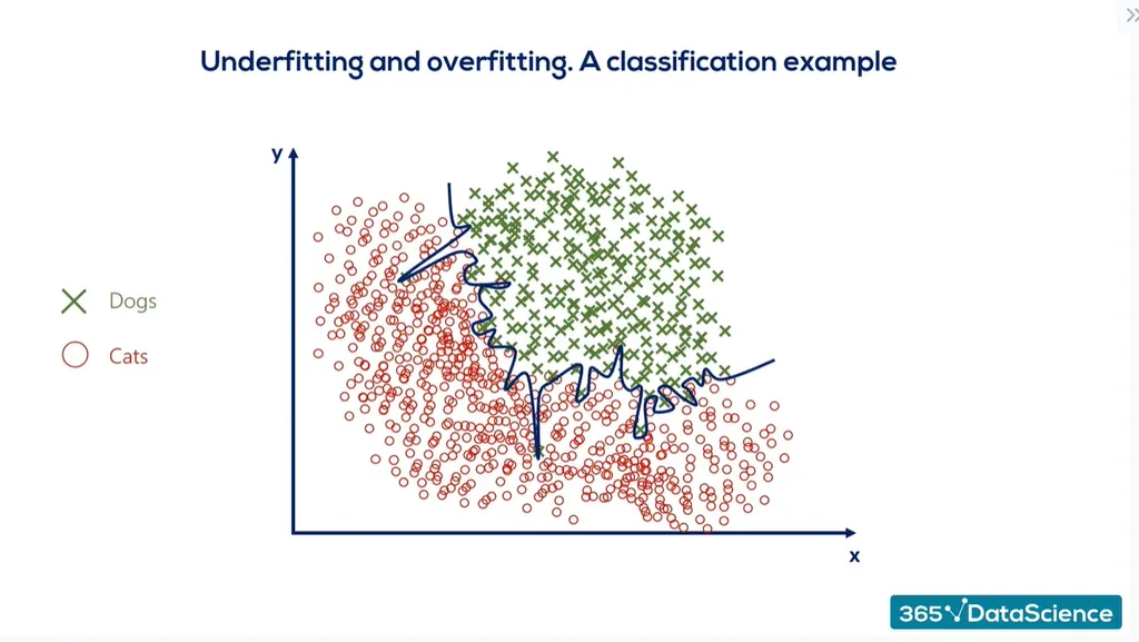
🔹 K = 1 (Overfitting, Very Detailed Boundaries)

- The model follows each individual data point closely.

- The boundary is highly irregular and sensitive to noise.

🔹 K = 3 (Balanced, Smooth but Still Detailed)

- The boundary is still detailed but less sensitive to small variations.

- Less overfitting than K=1.

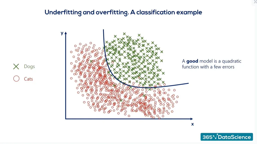
🔹 K = 5 (Smooth, More Generalized)

- The boundary becomes smoother.

- The model generalizes better but loses some fine details.

🔹 K = 10 (Underfitting, Too Simple)

- The boundary is very smooth and almost linear.

- The model underfits the data and loses key patterns.

3. Summary Table: Impact of K on Decision Boundary

K Value	Decision Boundary Shape	Effect
K = 1	Highly irregular, jagged	Overfits, memorizes training data
K = 3	Balanced, smooth but detailed	Good tradeoff between bias and variance
K = 5	Smooth and generalized	Less overfitting, better generalization
K = 10	Very smooth, almost linear	Underfits, loses details

4. Choosing the Best K?

- Use cross-validation to find the best K.

- A common rule of thumb: K = sqrt(N) (square root of the dataset size).

- If data is noisy, use a higher K to smooth out fluctuations.

5. Conclusion

📌 Small K (1, 3, 5) → Complex, detailed boundaries, but may overfit.

📌 Large K (20, 50, 100) → Smooth, generalized boundaries, but may underfit.

📌 Best K? → Found using cross-validation.

Understanding Overfitting and Underfitting

📌 What is Underfitting?

Figure: Underfitting - Model is too simple to capture patterns.

Underfitting happens when the model is too simple to learn patterns from data.

It performs poorly on both training and test data.

Example: Using K=100 in KNN creates a decision boundary that is too smooth, missing key details.

Analogy: A student who doesn’t study and guesses answers.

📌 What is Overfitting?

Figure: Overfitting - Model memorizes noise and outliers.

Overfitting happens when the model is too complex and memorizes data instead of generalizing.

It performs very well on training data but fails on test data.

Example: Using K=1 in KNN, the model follows every noise in data.

Analogy: A student who memorizes answers but fails new questions.

✅ The Ideal Model (Good Fit)

Figure: Overfitting - Model memorizes noise and outliers.

The best model balances complexity and generalization.

It performs well on both training and test data without overfitting or underfitting.

Example: Choosing K=5 or K=10 in KNN gives a smooth but useful decision boundary.

Analogy: A student who understands concepts instead of memorizing.

What is the Train Time Complexity of KNN & KD-Tree?

For KNN (K-Nearest Neighbors):

- Training space complexity: O(nd)
- Training time complexity: O(nd)
- Testing/Run time complexity: O(n * k * d), where:
    - n is the number of data points
    - k is the number of nearest neighbors considered
    - d is the number of dimensions/features

What are the assumptions of KNN ?

The KNN algorithm assumes that similar things exist in close proximity. In other words, similar things are near to each other.

KNN’s main disadvantage of becoming significantly slower as the volume of data increases makes it an impractical choice in environments where predictions need to be made rapidly.
Moreover, there are faster algorithms that can produce more accurate classification and regression results.

What happens if we do not normalize our dataset before classification using KNN ?

The k-nearest neighbor algorithm relies on majority voting based on class membership of 'k' nearest samples for a given test point. The nearness of samples is typically based on Euclidean distance. Feature scaling refers to the methods used to normalize the range of values of independent variables. In other words, the ways to set the feature value range within a similar scale. Feature magnitude matters for several reasons:

The scale of the variable directly influences the classification coefficient.

Variables with a more significant magnitude dominate over the ones with a smaller magnitude range.

Euclidean distances are sensitive to feature magnitude.

To overcome this effect, all features have to be at the same level of scale , especially for distance based algorithms

How is Weighted KNN Algorithm Better than Simple KNN Algorithm?

Issue with KNN: simplest method is to take the majority vote, but this can be a problem if the nearest neighbors vary widely in their distance and the closest neighbors more reliably indicate the class of the object.

1. Weighted KNN:

Weighted KNN assigns weights to the neighbors based on their distance to the query point. The weight can be inversely proportional to the distance, so closer neighbors have more influence on the prediction.

2. Advantages of Weighted KNN:

🔹 More accurate predictions by giving more weight to closer neighbors.
🔹 Reduces the impact of outliers and noisy data points.
🔹 Improves the performance of KNN in cases where the nearest neighbors are not equally reliable.

3. Weighted KNN Formula:

The weighted prediction is calculated as:

Weighted Prediction = \( \frac{\sum_{i=1}^{k} w_i \times
                                        y_i}{\sum_{i=1}^{k} w_i} \)

Where:

\( w_i \) is the weight assigned to the ith neighbor based on its distance.
\( y_i \) is the class label of the ith neighbor.
\( k \) is the number of neighbors considered.

4. Conclusion:

Weighted KNN is a more sophisticated version of the KNN algorithm that improves prediction accuracy by considering the reliability of each neighbor based on its distance to the query point.

k in k-NN in Terms of Bias

Which of the following will be true about k in k-NN in terms of Bias?

A) When you increase the k, the bias will increase ✅
B) When you decrease the k, the bias will increase ❌
C) Can’t say ❌
D) None of these ❌

Solution: A) A large K means a simpler model, and a simpler model is always considered to have high bias.

Which of the following will be true about k in k-NN in terms of Variance?

A) When you increase the k, the variance will increase ❌
B) When you decrease the k, the variance will increase ✅
C) Can’t say ❌
D) None of these ❌

Solution: B) A simple model is considered a low variance model, meaning that when k decreases, variance increases.