Performance Metrics

Performance Metrics in Machine Learning

1. Accuracy

Definition: Accuracy is the ratio of correctly predicted instances to the total number of instances.

Formula: Accuracy = (TP + TN) / (TP + TN + FP + FN)

Example:

A model classifies 100 patients as having or not having a disease.

  • TP = 50 (Correctly detected as positive)
  • TN = 30 (Correctly detected as negative)
  • FP = 10 (Healthy but wrongly classified as sick)
  • FN = 10 (Sick but wrongly classified as healthy)

Accuracy = (50 + 30) / (50 + 30 + 10 + 10) = 80%

Limitation: In imbalanced datasets (e.g., 95% class A, 5% class B), a model predicting only class A will have high accuracy but fail for class B.

2. Precision

Definition: Precision measures how many of the predicted positive cases are actually correct.

Formula: Precision = TP / (TP + FP)

Example:

In a spam detection model:

  • TP = 40 (Correctly identified spam emails)
  • FP = 20 (Non-spam emails mistakenly marked as spam)

Precision = 40 / (40 + 20) = 0.67 (67%)

Use case: When false positives must be minimized, such as spam detection.

3. Recall (Sensitivity)

Definition: Recall measures how many actual positive cases were correctly predicted.

Formula: Recall = TP / (TP + FN)

Example:

In a cancer detection model:

  • TP = 45 (Correctly identified cancer patients)
  • FN = 5 (Cancer patients incorrectly classified as healthy)

Recall = 45 / (45 + 5) = 0.90 (90%)

Use case: Important in medical diagnosis where missing a positive case can be critical.

4. F1-Score

Definition: The F1-score is the harmonic mean of precision and recall.

Formula: F1 = 2 × (Precision × Recall) / (Precision + Recall)

Example:

For a model with:

  • Precision = 0.67
  • Recall = 0.90

F1 = 2 × (0.67 × 0.90) / (0.67 + 0.90) = 0.76 (76%)

Use case: Useful for imbalanced datasets where both false positives and false negatives are important.

5. ROC-AUC Score

Definition: The Receiver Operating Characteristic (ROC) curve plots the True Positive Rate (TPR) against the False Positive Rate (FPR) at various threshold settings.

Formula: ROC-AUC measures the area under this curve, with values closer to 1 being better.

Example:

Consider two models:

  • Model A has an ROC-AUC of 0.95
  • Model B has an ROC-AUC of 0.75

Model A is better at distinguishing between positive and negative cases.

Use case: Useful for evaluating classification models with probability scores.

6. Log Loss (Logarithmic Loss)

Definition: Log Loss measures the difference between predicted probabilities and actual labels.

Formula: Log Loss = - (1/N) Σ (y log(p) + (1-y) log(1-p))

Example:

If a model predicts probabilities for five samples:

  • True labels: [1, 0, 1, 1, 0]
  • Predicted probabilities: [0.9, 0.1, 0.8, 0.7, 0.2]

The log loss will be low, indicating good predictions.

Use case: Commonly used in probabilistic models like logistic regression.

Comparison Table

Metric Formula Example Use Case Limitations
Accuracy (TP + TN) / (TP + TN + FP + FN) General classification Misleading for imbalanced datasets
Precision TP / (TP + FP) Spam filtering Ignores false negatives
Recall TP / (TP + FN) Medical diagnosis Ignores false positives
F1-Score 2 × (Precision × Recall) / (Precision + Recall) Imbalanced datasets Harder to interpret than accuracy
ROC-AUC Area under the ROC curve Evaluating probabilistic classifiers Not useful for multi-class classification
Log Loss - (1/N) Σ (y log(p) + (1-y) log(1-p)) Probabilistic classification Hard to interpret directly

Conclusion

  • ✅ Use Accuracy when the dataset is balanced.
  • ✅ Use Precision when false positives must be minimized.
  • ✅ Use Recall when false negatives must be minimized.
  • ✅ Use F1-Score for imbalanced datasets.
  • ✅ Use ROC-AUC for probability-based models.
  • ✅ Use Log Loss for probabilistic classification.

Can We Use Accuracy for Imbalanced Data?

Is Accuracy a Good Metric for Imbalanced Data?

Accuracy is not always the best metric for evaluating classification models, especially when dealing with imbalanced datasets. In such cases, other metrics like Precision, Recall, and F1-Score provide a better assessment of model performance.

Example: Flight Accident Data

Consider a dataset that predicts whether a flight Landed Safely (1) or Crashed (0).

  • 90% of flights land safely
  • 10% of flights crash

If a model predicts every flight as "Landed Safely (1)", it would still achieve 90% accuracy, even though it completely fails to detect any crashes. This makes accuracy a misleading metric in such cases.

Why Accuracy is Not Reliable for Imbalanced Data

  • Does not consider class distribution: When one class is dominant, accuracy remains high even if the model fails to predict the minority class.
  • Fails in real-world applications: In critical fields like fraud detection or medical diagnosis, missing minority class predictions can have severe consequences.
  • Ignores false positives and false negatives: A model with high accuracy may still have a high error rate in predicting minority class instances.

Better Alternatives to Accuracy

  • Precision: Measures how many of the predicted positive cases were actually positive.
  • Recall: Measures how many actual positive cases were correctly identified.
  • F1-Score: A balanced metric that combines Precision and Recall.
  • ROC-AUC: Evaluates the trade-off between sensitivity and specificity.

Conclusion

For highly imbalanced datasets, accuracy is often misleading. Instead, metrics like Recall, Precision, and F1-Score provide a clearer picture of model performance, especially in cases where the minority class is critical.

Inputs Required to Calculate Average F1 Score

The inputs required to calculate the average F1 Score are:

  • TP (True Positives): Correctly predicted positive cases.
  • FP (False Positives): Incorrectly predicted positive cases.
  • FN (False Negatives): Incorrectly predicted negative cases.

Steps to Compute Average F1 Score

1. Calculate Precision for each class

Precision measures how many of the predicted positive cases are actually correct.

Formula:

Precision = TP / (TP + FP)

2. Calculate Recall for each class

Recall measures how many actual positive cases were correctly predicted.

Formula:

Recall = TP / (TP + FN)

3. Calculate F1 Score for each class

The F1 Score is the harmonic mean of Precision and Recall.

Formula:

F1 = 2 × (Precision × Recall) / (Precision + Recall)

Types of Average F1 Score

1. Macro F1 Score

Macro F1 Score is the unweighted mean of the F1 Scores of all classes.

Formula:

Macro F1 = (F11 + F12 + ... + F1n) / n

Use case: Suitable when all classes should be treated equally.

2. Weighted F1 Score

Weighted F1 Score considers the number of instances in each class.

Formula:

Weighted F1 = Σ (Samples in class × F1) / Total Samples

Use case: Useful when classes are imbalanced.

3. Micro F1 Score

Micro F1 Score computes global TP, FP, and FN across all classes before calculating F1.

Formula:

Micro F1 = 2 × (Σ TP) / (2 × Σ TP + Σ FP + Σ FN)

Use case: Preferred when class distribution is imbalanced and you want to evaluate overall performance.

Conclusion

  • Use Macro F1 when you want to treat all classes equally.
  • Use Weighted F1 when dealing with imbalanced datasets.
  • Use Micro F1 when evaluating overall classification performance.

Inputs Required to Calculate Average F1 Score

The inputs required to calculate the average F1 Score are:

  • TP (True Positives): Correctly predicted positive cases.
  • FP (False Positives): Incorrectly predicted positive cases.
  • FN (False Negatives): Incorrectly predicted negative cases.

Example: Multi-Class Classification

Consider a classification model that predicts three classes: Cat, Dog, Rabbit.

Class TP FP FN
Cat 50 10 5
Dog 40 20 15
Rabbit 30 5 10

Step 1: Calculate Precision & Recall for Each Class

For Cat:

  • Precision = TP / (TP + FP) = 50 / (50 + 10) = 0.833
  • Recall = TP / (TP + FN) = 50 / (50 + 5) = 0.909

For Dog:

  • Precision = 40 / (40 + 20) = 0.667
  • Recall = 40 / (40 + 15) = 0.727

For Rabbit:

  • Precision = 30 / (30 + 5) = 0.857
  • Recall = 30 / (30 + 10) = 0.750

Step 2: Calculate F1 Score for Each Class

For Cat:

F1 = 2 × (0.833 × 0.909) / (0.833 + 0.909) = 0.869

For Dog:

F1 = 2 × (0.667 × 0.727) / (0.667 + 0.727) = 0.696

For Rabbit:

F1 = 2 × (0.857 × 0.750) / (0.857 + 0.750) = 0.800

Step 3: Compute the Average F1 Score

1. Macro F1 Score (Unweighted Average)

Macro F1 = (0.869 + 0.696 + 0.800) / 3 = 0.788

2. Weighted F1 Score

Weighted F1 = (55 × 0.869 + 55 × 0.696 + 40 × 0.800) / (55 + 55 + 40) = 0.778

3. Micro F1 Score

Micro F1 = 2 × (Σ TP) / (2 × Σ TP + Σ FP + Σ FN)

= 2 × (50 + 40 + 30) / (2 × (50 + 40 + 30) + (10 + 20 + 5) + (5 + 15 + 10))

= 2 × (120) / (2 × 120 + 35 + 30) = 240 / 275 = 0.873

Conclusion

  • Macro F1 Score: 0.788 (Treats all classes equally)
  • Weighted F1 Score: 0.778 (Gives more weight to larger classes)
  • Micro F1 Score: 0.873 (Balances overall performance)

Recall is More Important than Precision (and Vice Versa)

The importance of recall versus precision depends on the specific problem and the consequences of false positives versus false negatives.

When Recall is More Important

Recall is crucial when missing a positive instance (false negative) is more costly than incorrectly flagging some negative instances (false positives).

  • Medical Diagnoses: In diseases like cancer detection or COVID-19 testing, missing a positive case could be life-threatening, so high recall is preferred.
  • Fraud Detection: Banks and financial institutions prioritize recall to catch as many fraudulent transactions as possible, even if it means investigating some false alarms.
  • Search Engines & Information Retrieval: It’s better to show more search results (even with some irrelevant ones) than to miss valuable information.
  • Fire Alarm Systems: Missing a fire could be catastrophic, so it's better to raise a few false alarms than to miss a real fire.
  • Crime Surveillance: Security cameras analyzing threats should aim for high recall to avoid missing potential dangers.
  • Disaster Warning Systems: Early warnings for tsunamis, earthquakes, or hurricanes must prioritize recall to avoid missing real threats.

When Precision is More Important

Precision is critical when false positives (incorrectly classifying negatives as positives) are more problematic than missing some positive instances.

  • Spam Detection: If a legitimate email is incorrectly flagged as spam, it may cause users to miss important messages.
  • Autonomous Vehicles: A false alarm causing unnecessary braking could be dangerous, so precision is prioritized in object detection.
  • Online Advertising: Displaying ads to uninterested users wastes resources, so precision is crucial.
  • Drug Approval: Approving a harmful drug (false positive) is much worse than rejecting a potentially useful one.
  • Customer Support Chatbots: Incorrect automated responses reduce user trust, so precision is emphasized.

When a Balance is Needed

In some scenarios, both false positives and false negatives have significant consequences, making it essential to find a balance between recall and precision.

  • Recommendation Systems: Missing a good recommendation (false negative) is bad, but showing too many irrelevant ones (false positive) also affects user engagement.
  • Fraud Detection in Banking: While high recall is necessary, too many false positives (flagging legitimate transactions) can frustrate customers.
  • Sentiment Analysis: In business decisions, incorrectly classifying customer sentiment can lead to misguided strategies.

Conclusion

Choosing between recall and precision depends on the problem at hand. In life-critical systems (e.g., medical diagnoses, disaster warnings), recall is prioritized. In systems where incorrect classifications cause harm (e.g., spam filters, hiring decisions), precision is more important. When both false positives and false negatives matter, a balance between the two is required using metrics like the F1 Score.

When is Precision More Important Over Recall?

Understanding Precision vs. Recall

  • Precision: When the model predicts a positive case, how often is it actually correct?
  • Recall: Out of all actual positive cases, how many did the model correctly identify?

When Precision is More Important?

Precision is prioritized when false positives are more costly or dangerous than false negatives.

Example 1: Spam Email Detection

  • If an email is falsely classified as spam (false positive), an important message might be lost.
  • It is acceptable to let a few spam emails (false negatives) reach the inbox, rather than marking important emails as spam.
  • Priority: High precision ensures only actual spam emails are marked.

Example 2: Fraud Detection

  • Blocking a genuine transaction (false positive) can frustrate customers.
  • It is better to allow some fraudulent transactions (false negatives) rather than mistakenly blocking too many legitimate ones.
  • Priority: High precision prevents false fraud alerts.

Example 3: Medical Diagnosis (Non-Life-Threatening Diseases)

  • Consider a test for mild allergies.
  • If a person is incorrectly diagnosed as allergic (false positive), they may unnecessarily avoid certain foods.
  • However, missing a real allergy (false negative) is not life-threatening.
  • Priority: High precision ensures fewer people are wrongly diagnosed.

Conclusion

Choose precision over recall when the cost of a false positive is higher than a false negative.

  • Spam detection: Avoid marking good emails as spam.
  • Fraud detection: Prevent blocking real transactions.
  • Medical diagnosis: Prevent unnecessary panic from wrong results.

When is Recall More Important Over Precision?

Understanding Recall vs. Precision

  • Recall: Out of all actual positive cases, how many did the model correctly identify?
  • Precision: When the model predicts a positive case, how often is it actually correct?

When Recall is More Important?

Recall is prioritized when false negatives are more costly or dangerous than false positives.

Example 1: Medical Diagnosis (Life-Threatening Diseases)

  • In diseases like cancer, missing a real case (false negative) can delay treatment and be life-threatening.
  • It is better to have a few false alarms (false positives) than to miss actual patients.
  • Priority: High recall ensures all potential cases are detected.

Example 2: Fraud Detection

  • Allowing a fraudulent transaction (false negative) can cause financial loss.
  • It's okay to flag some legitimate transactions (false positives) if it means catching all fraudulent ones.
  • Priority: High recall minimizes undetected fraud.

Example 3: Fire or Intrusion Detection

  • If a fire or burglary alarm fails to trigger (false negative), the consequences can be severe.
  • It's acceptable to have some false alarms (false positives) rather than missing a real emergency.
  • Priority: High recall ensures every real emergency is detected.

Example 4: Search Engines & Information Retrieval

  • A search engine should return all relevant documents (high recall), even if some irrelevant ones appear.
  • Missing important search results (false negatives) is worse than showing a few extra ones.
  • Priority: High recall improves user experience.

Conclusion

Choose recall over precision when missing a positive case is riskier than a false alarm.

  • Medical diagnosis: Detect all possible patients.
  • Fraud detection: Catch all fraudulent activities.
  • Security systems: Never miss a fire or burglary alert.
  • Search engines: Retrieve all relevant results.

What is Cross-Validation and Why is it Needed?

1. What is Cross-Validation?

Cross-validation (CV) is a technique used in machine learning and statistics to evaluate the performance of a model on unseen data. Instead of using a single train-test split, cross-validation splits the dataset multiple times to ensure the model generalizes well.

2. Why is Cross-Validation Needed?

  • Avoids Overfitting: It prevents models from being too specific to the training data and ensures they perform well on new data.
  • More Reliable Performance Metrics: Instead of depending on a single test set, multiple validations provide a better estimate of model accuracy.
  • Efficient Use of Data: Useful when you have limited data, as it allows every sample to be used for training and testing.
  • Hyperparameter Tuning: Helps in selecting the best model parameters using techniques like Grid Search or Random Search.

3. Types of Cross-Validation

  • K-Fold Cross-Validation:
    • The dataset is split into K equal-sized folds (e.g., K=5).
    • The model is trained on K-1 folds and tested on the remaining fold.
    • This process is repeated K times, with each fold used once for testing.
    • The final performance is the average of all K iterations.
  • Stratified K-Fold Cross-Validation:
    • Similar to K-Fold but ensures class distribution remains consistent across all folds.
    • Useful for imbalanced datasets.
  • Leave-One-Out Cross-Validation (LOO-CV):
    • Each data point is used once as a test set, while the rest are used for training.
    • Computationally expensive but useful when the dataset is very small.
  • Leave-P-Out Cross-Validation (LPO-CV):
    • Similar to LOO-CV but leaves out P data points instead of just one.
    • Even more computationally expensive than LOO.
  • Time Series Cross-Validation (Rolling Window CV):
    • Used for time-dependent data (e.g., stock prices, weather forecasting).
    • Ensures that past data is used to predict future outcomes without data leakage.

4. When to Use Cross-Validation?

  • When you don’t have a large dataset and want to make the best use of available data.
  • When tuning hyperparameters to get the best model configuration.
  • When you need a reliable estimate of model performance before deploying it.

Conclusion

Cross-validation is an essential technique for evaluating machine learning models, ensuring they generalize well to new data. It prevents overfitting, improves reliability, and helps in model selection. Choosing the right type of cross-validation depends on the dataset and the problem at hand.

Difference Between One-Vs-Rest (OvR) and One-Vs-One (OvO)

Why Use OvR or OvO?

Not all classification algorithms support multi-class classification. Some algorithms, like the Perceptron, Logistic Regression, and Support Vector Machines (SVMs), are designed for binary classification.

To use these binary classifiers for multi-class problems, we split the dataset into multiple binary classification problems. Two common approaches are:

  • One-vs-Rest (OvR) or One-vs-All (OvA)
  • One-vs-One (OvO)

One-Vs-Rest (OvR) for Multi-Class Classification

One-vs-Rest (OvR) is a method where the multi-class dataset is split into multiple binary classification problems. Each classifier is trained to distinguish one class from all the others. The final prediction is made by the classifier that is most confident.

Example

Consider a dataset with three classes: red, blue, and green. The OvR approach creates the following binary classification problems:

  • Binary Classification Problem 1: red vs. [blue, green]
  • Binary Classification Problem 2: blue vs. [red, green]
  • Binary Classification Problem 3: green vs. [red, blue]

Advantages of One-Vs-Rest

  • Faster training since it requires only K models (where K is the number of classes).
  • Works well when one class is significantly different from others.

Disadvantages of One-Vs-Rest

  • Can be affected by imbalanced data (if one class has far fewer examples than others).
  • Predictions can be inconsistent when multiple classifiers give similar confidence scores.

One-Vs-One (OvO) for Multi-Class Classification

One-vs-One (OvO) is a method where the dataset is split into multiple binary classification problems, but instead of comparing one class against all others, it compares every pair of classes individually. The final prediction is made using a voting system among all classifiers.

Example

Consider a dataset with four classes: red, blue, green, and yellow. The OvO approach creates the following binary classification problems:

  • Binary Classification Problem 1: red vs. blue
  • Binary Classification Problem 2: red vs. green
  • Binary Classification Problem 3: red vs. yellow
  • Binary Classification Problem 4: blue vs. green
  • Binary Classification Problem 5: blue vs. yellow
  • Binary Classification Problem 6: green vs. yellow

Advantages of One-Vs-One

  • Better for models that don't scale well with large datasets (e.g., SVMs), since each classifier sees only two classes.
  • More accurate when classes are well-separated.

Disadvantages of One-Vs-One

  • Requires K(K-1)/2 models, making it computationally expensive.
  • Can be slow for large numbers of classes.

Comparison Table

Feature One-Vs-Rest (OvR) One-Vs-One (OvO)
Number of Classifiers K K(K-1)/2
Training Speed Faster Slower (more classifiers)
Inference Speed Faster Slower
Best for Large Datasets? Yes No
Best for Algorithms like SVM? No Yes
Accuracy Good, but may struggle with close decision boundaries. Higher, since each classifier focuses on two specific classes.

Conclusion

Both One-Vs-Rest and One-Vs-One are useful techniques for adapting binary classifiers to multi-class problems.

  • Use One-Vs-Rest: When you need faster training and have a large dataset.
  • Use One-Vs-One: When using SVMs or when higher accuracy is needed, even if it is computationally expensive.

Mean Average Precision (mAP)?

1. Understanding Average Precision (AP)

Average Precision (AP) measures the area under the Precision-Recall (PR) curve. It evaluates how well a classification or object detection model balances precision and recall.

2. What is Mean Average Precision (mAP)?

Mean Average Precision (mAP) is the average of AP scores across all categories in a dataset. It is commonly used in object detection and information retrieval tasks.

Mathematically, mAP is calculated as:

mAP = (AP₁ + AP₂ + ... + APₙ) / N

where:

  • AP₁, AP₂, ..., APₙ are the average precision values for each class.
  • N is the total number of classes.

3. How is mAP Used?

mAP is widely used in:

  • Object Detection: Evaluating models like YOLO, Faster R-CNN, and SSD.
  • Information Retrieval: Measuring ranking effectiveness in search engines.
  • Recommendation Systems: Assessing ranking quality of suggested items.

4. Why is mAP Important?

  • Balances Precision & Recall: Unlike accuracy, mAP considers both false positives and false negatives.
  • Useful for Imbalanced Data: Works well even when some classes are underrepresented.
  • Standard Benchmark: Common metric in computer vision and ranking tasks.

5. Conclusion

mAP provides a robust evaluation metric for tasks where ranking and precision-recall trade-offs matter. It is a key metric in object detection, retrieval systems, and recommendation engines.

Best Performance Metric for Highly Imbalanced Data

1. Understanding the Problem

When dealing with a dataset where the number of positive samples (minority class) is much lower than the number of negative samples (majority class), traditional metrics like accuracy become unreliable.

2. Why Precision is a Better Choice?

If the dataset is highly imbalanced, precision is a more suitable metric because:

  • Precision measures the proportion of true positives among all predicted positives:
    Precision = TP / (TP + FP)
  • It is not affected by the large number of negative samples, unlike False Positive Rate (FPR).
  • It focuses on the correct detection of the minority class (positive class).

3. Why Not Use False Positive Rate (FPR)?

False Positive Rate (FPR) is defined as:

FPR = FP / (FP + TN)

When the number of negative samples (TN) is very large, FPR remains low even if the model makes many false positives, making it a less reliable metric.

4. Alternative Metrics for Imbalanced Data

Besides precision, other useful metrics include:

  • Recall: Measures how many actual positives were correctly identified.
  • F1-Score: Harmonic mean of Precision and Recall, balancing both.
  • Precision-Recall (PR) Curve: More informative than ROC in highly imbalanced cases.
  • ROC-AUC: Measures the model's ability to distinguish between classes.

5. Conclusion

For datasets with a large number of negative samples, precision is a better metric than FPR because it focuses on the correct identification of positive cases without being affected by the abundance of negative samples.

Few Scenarios

Example 1.a: Majority Positive Samples – All Detected, But False Positives Exist

Dataset: 9 positive samples, 1 negative sample.

Model Prediction: Predicts all samples as positive.

  • TP = 9, FP = 1, TN = 0, FN = 0
  • Precision = 9/10 = 0.9, Recall = 9/9 = 1.0
  • TPR = 1.0, FPR = 1.0

Since FPR is very high, the model is not reliable despite high precision and recall. ROC is a better metric here.

Example 1.b: Opposite Labels – No Detection

Dataset: 9 negative samples, 1 positive sample.

Model Prediction: Predicts all as negative.

  • TP = 0, FP = 0, TN = 9, FN = 1
  • Precision, Recall, TPR, and FPR are all 0.

This model fails entirely.

Example 2.a: Majority Positive Samples – All Detected, Some False Positives

Dataset: 8 positive samples, 2 negative samples.

Model Prediction: Predicts 9 as positive, 1 as negative.

  • TP = 8, FP = 1, TN = 1, FN = 0
  • Precision = 8/9 = 0.89, Recall = 1.0
  • TPR = 1.0, FPR = 0.5

FPR is high (0.5), showing poor performance for negative class. ROC is better in this case.

Example 2.b: Opposite Labels

Dataset: 8 negative samples, 2 positive samples.

Model Prediction: Predicts 1 as positive, rest as negative.

  • TP = 1, FP = 0, TN = 8, FN = 1
  • Precision = 1.0, Recall = 0.5
  • TPR = 0.5, FPR = 0

Low recall (0.5) but good precision.

Example 3.a: Majority Positive Samples – Some Missed

Dataset: 9 positive samples, 1 negative sample.

Model Prediction: Predicts 7 as positive, 3 as negative.

  • TP = 7, FP = 0, TN = 1, FN = 2
  • Precision = 1.0, Recall = 7/9 = 0.78
  • TPR = 0.78, FPR = 0

Both metrics indicate strong performance.

Example 3.b: Opposite Labels – Precision and Recall Are Better

Dataset: 9 negative samples, 1 positive sample.

Model Prediction: Predicts 3 as positive (1 correct), 7 as negative.

  • TP = 1, FP = 2, TN = 7, FN = 0
  • Precision = 1/3 = 0.33, Recall = 1.0
  • TPR = 1.0, FPR = 2/9 = 0.22

FPR is low, but poor detection is reflected in low precision.

Final Conclusion: Choosing the Right Metric

  • Use Precision & Recall: When the positive class is small and detecting positives is the priority.
  • Use ROC: When both classes are equally important.
  • Use ROC for Majority Positives: Since precision and recall focus mostly on the positive class.
  • Switch Labels: If the minority class is more important, swap labels and use precision & recall.

Regularization in Machine Learning

Regularization is a technique used to prevent overfitting in machine learning models. Overfitting occurs when a model learns the training data too well, including noise and outliers, and performs poorly on unseen data. Regularization introduces additional constraints or penalties to the model's learning process to ensure it generalizes better to new data.

Why Regularization is Needed

  • Overfitting: Models with high complexity may fit training data perfectly but fail on new data.
  • High Variance: Overfit models are sensitive to small fluctuations in training data.
  • Regularization balances the trade-off between bias (underfitting) and variance (overfitting).

Types of Regularization

1. L1 Regularization (Lasso Regression)

  • Concept: Adds a penalty equal to the absolute value of the coefficients.
  • Effect: Encourages sparsity by shrinking some coefficients to zero, performing feature selection.

2. L2 Regularization (Ridge Regression)

  • Concept: Adds a penalty equal to the square of the coefficients.
  • Effect: Shrinks all coefficients proportionally but does not set them to zero.

3. Elastic Net Regularization

  • Concept: Combines L1 and L2 regularization.
  • Effect: Balances the benefits of both L1 and L2 regularization.

4. Dropout (for Neural Networks)

  • Concept: Randomly ignores a fraction of neurons during training.
  • Effect: Reduces co-adaptation of neurons, making the network more robust.

5. Early Stopping

  • Concept: Stops training when validation performance degrades.
  • Effect: Prevents the model from learning noise in the training data.

Key Concepts in Regularization

  • Regularization Parameter (λ): Controls the strength of regularization.
  • Bias-Variance Trade-off: Regularization introduces bias to reduce variance.
  • Feature Selection: L1 regularization can shrink some coefficients to zero.

When to Use Regularization

  • When the model is overfitting (high variance).
  • When the dataset has high dimensionality (many features).
  • When there is multicollinearity (correlated features).

Advantages of Regularization

  • Improves generalization to unseen data.
  • Reduces model complexity.
  • Helps handle multicollinearity.
  • Can perform feature selection (L1 regularization).

Disadvantages of Regularization

  • Introduces bias into the model.
  • Requires tuning of the regularization parameter (λ).
  • May not always improve performance if the model is already simple.

Conclusion

Regularization is a powerful tool to prevent overfitting and improve the generalization of machine learning models. By adding a penalty to the loss function, it balances the trade-off between bias and variance, ensuring the model performs well on both training and unseen data. The choice of regularization technique (L1, L2, Elastic Net, etc.) depends on the specific problem and dataset.

Bias-Variance Tradeoff

In order to understand how the deviation of the function is varied, bias and variance can be adopted. Bias is the measurement of deviation or error from the real value of the function, while variance is the measurement of deviation in the response variable function when estimating it over different training samples of the dataset.

Therefore, for a generalized data model, we must keep bias as low as possible to achieve high accuracy. Additionally, the model should not produce greatly varied results, so low variance is recommended for good performance.

The relationship between bias and variance is closely related to overfitting, underfitting, and model capacity. When calculating the generalization error (where bias and variance are crucial elements), an increase in model capacity can lead to an increase in variance and a decrease in bias.

The trade-off is the tension between the error introduced by bias and variance. The image below shows the bias-variance tradeoff as a function of model capacity.

Bias-Variance Tradeoff Graph

From the graph, it can be observed that:

  • While reducing bias, the model fits well on a particular sample of training data but fails to generalize to unseen data, leading to high variance.
  • If we aim to keep variance low, the model may not fit the data well, resulting in high bias.

Graphical Representation of Underfitting, Exact Fit, and Overfitting

The graph below depicts the conditions of underfitting, exact fit, and overfitting.

Examples of Bias-Variance Tradeoff

  • Support Vector Machine (SVM): Has low bias and high variance. The trade-off can be altered by increasing the cost (C) parameter, which decreases variance and increases bias.
  • k-Nearest Neighbors (k-NN): Has low bias and high variance. The trade-off can be modified by increasing the k-value, which increases bias.

Overfitting and Underfitting

Overfitting occurs when a model has low bias and high variance, fitting the training data too well but failing to generalize to new data. This often happens when the model considers too many features, including insignificant ones.

Underfitting occurs when a model has high bias and low variance, failing to capture the underlying patterns in the data.

What is Regularization?

Regularization is a technique used to prevent overfitting by penalizing complex models. It achieves this by adding a regularization term to the loss function, which shrinks the model's coefficients towards zero. This reduces the impact of insignificant features and stabilizes the model.

Regularization Techniques

  • L1 Regularization (Lasso): Adds a penalty equal to the absolute value of the coefficients. It encourages sparsity and performs feature selection.
  • L2 Regularization (Ridge): Adds a penalty equal to the square of the coefficients. It shrinks all coefficients but does not set them to zero.
  • Elastic Net: Combines L1 and L2 regularization.
  • Dropout: Randomly ignores neurons during training in neural networks.
  • Early Stopping: Stops training when validation performance degrades.

Regularization Term

Regularization adds a penalty term to the cost function to penalize complex models. This reduces the weights of the model, making it simpler and less prone to overfitting.

Penalty Terms

  • L1 Penalty: Adds the absolute value of coefficients (used in Lasso Regression).
  • L2 Penalty: Adds the squared value of coefficients (used in Ridge Regression).
  • Elastic Net: Combines L1 and L2 penalties.

L1 Regularization

L1 regularization is preferred when dealing with high-dimensional data, as it provides sparse solutions by shrinking some coefficients to zero. The regression model using L1 regularization is called Lasso Regression.

Mathematical Formula for L1 Regularization

The loss function with L1 regularization is:

\[ \text{Loss} = \text{Error}(Y, \hat{Y}) + \lambda \sum_{i=1}^n |w_i| \]

Where \( \lambda \) is the regularization parameter.

L2 Regularization

L2 regularization is used to handle multicollinearity by shrinking all coefficients proportionally. The regression model using L2 regularization is called Ridge Regression.

Mathematical Formula for L2 Regularization

The loss function with L2 regularization is:

\[ \text{Loss} = \text{Error}(Y, \hat{Y}) + \lambda \sum_{i=1}^n w_i^2 \]

L1 vs L2 Regularization

Key differences between L1 and L2 regularization:

  • L1: Produces sparse solutions, performs feature selection, and is robust to outliers.
  • L2: Produces non-sparse solutions, does not perform feature selection, and is computationally efficient.

Conclusion

Regularization is a powerful technique to prevent overfitting by penalizing complex models. L1 regularization is useful for feature selection, while L2 regularization is better for handling multicollinearity. The choice between L1 and L2 depends on the specific problem and dataset.

Why L1 Regularization Creates Sparsity in the Weight Vector

1. Mathematical Formulation

L1 Regularization (Lasso):

The loss function with L1 regularization is:

\[ \mathcal{L}_1 = \text{Logistic Loss} + \lambda \sum_{i=1}^d |W_i| \]

The gradient of the L1 penalty is:

\[ \frac{\partial \mathcal{L}_1}{\partial W_i} = \begin{cases} +\lambda & \text{if } W_i > 0 \\ -\lambda & \text{if } W_i < 0 \end{cases} \]

L2 Regularization (Ridge):

The loss function with L2 regularization is:

\[ \mathcal{L}_2 = \text{Logistic Loss} + \lambda \sum_{i=1}^d W_i^2 \]

The gradient of the L2 penalty is:

\[ \frac{\partial \mathcal{L}_2}{\partial W_i} = 2\lambda W_i \]

2. Gradient Descent Behavior

L1 Regularization:

  • Weight update rule: \[ W_i^{(t+1)} = W_i^{(t)} - \eta \left( \frac{\partial \text{Logistic Loss}}{\partial W_i} + \lambda \cdot \text{sign}(W_i) \right) \]
  • The L1 penalty subtracts a fixed value (\(\eta \lambda\)) from \(W_i\) at each step, regardless of its magnitude.
  • Small weights can be pushed past zero, leading to exact sparsity.

L2 Regularization:

  • Weight update rule: \[ W_i^{(t+1)} = W_i^{(t)} - \eta \left( \frac{\partial \text{Logistic Loss}}{\partial W_i} + 2\lambda W_i \right) \]
  • The L2 penalty shrinks \(W_i\) proportionally to its current value (\(2\lambda W_i\)).
  • Small weights are reduced slightly but never reach zero.

3. Geometric Interpretation

L1 Constraint (Diamond Shape):

  • The feasible region is a polyhedron with corners on the axes.
  • Optimal solutions often lie at corners where weights are exactly zero.

L2 Constraint (Sphere Shape):

  • The feasible region is a smooth sphere.
  • Optimal solutions rarely lie on the axes, resulting in non-sparse weights.

4. Example: Gradient Descent Updates

Assume \(W_1 = 0.1\), \(\lambda = 0.1\), and \(\eta = 0.01\):

L1 Regularization:

  • Gradient of penalty: \(\frac{\partial \mathcal{L}_1}{\partial W_1} = +0.1\) (since \(W_1 > 0\)).
  • Update: \(W_1 \leftarrow 0.1 - 0.01 \times 0.1 = 0.099\).
  • Repeated updates drive \(W_1\) to 0.

L2 Regularization:

  • Gradient of penalty: \(\frac{\partial \mathcal{L}_2}{\partial W_1} = 2 \times 0.1 \times 0.1 = 0.02\).
  • Update: \(W_1 \leftarrow 0.1 - 0.01 \times 0.02 = 0.0998\).
  • \(W_1\) shrinks gradually but never reaches zero.

5. Comparison Table

Aspect L1 Regularization L2 Regularization
Gradient Constant (\(\pm \lambda\)) Proportional to \(W_i\) (\(2\lambda W_i\))
Sparsity Yes (weights reach exactly zero) No (weights remain non-zero)
Use Case Feature selection, high-dimensional data Handling multicollinearity

Conclusion

L1 regularization creates sparsity because:

  1. Its constant gradient pushes small weights past zero during updates.
  2. The non-differentiable "kink" at zero traps weights at zero.
  3. Geometric constraints favor corner solutions with sparse weights.

L2 regularization, in contrast, shrinks weights smoothly but never achieves exact sparsity.

Bias-Variance Tradeoff

1. Definitions

  • Bias:
    • Error from erroneous assumptions in the learning algorithm.
    • High bias causes underfitting (model misses relevant patterns in data).
  • Variance:
    • Error from sensitivity to small changes in the training set.
    • High variance causes overfitting (model learns noise and fails on unseen data).

2. Goal of Model Selection

Choose a model that:

  1. Accurately captures patterns in training data.
  2. Generalizes well to unseen data.

Key Challenge: Balancing these goals is often contradictory.

3. Tradeoff Dynamics

  • High-Variance Models:
    • Complex models (e.g., deep neural networks).
    • Excel on training data but overfit to noise.
    • Poor test performance.
  • High-Bias Models:
    • Simple models (e.g., linear regression).
    • Underfit by missing key patterns.
    • Consistent but inaccurate predictions.

4. Impact of Model Complexity

  • Increased Complexity:
    • Reduces bias (captures more patterns).
    • Increases variance (sensitive to noise).
    • Example: Flexible model \( \hat{f}(x) \) fits training data closely but overfits.
  • Reduced Complexity:
    • Increases bias (misses patterns).
    • Reduces variance (stable predictions).
    • Example: Rigid model ignores subtle relationships.
Bias-Variance Tradeoff Graph

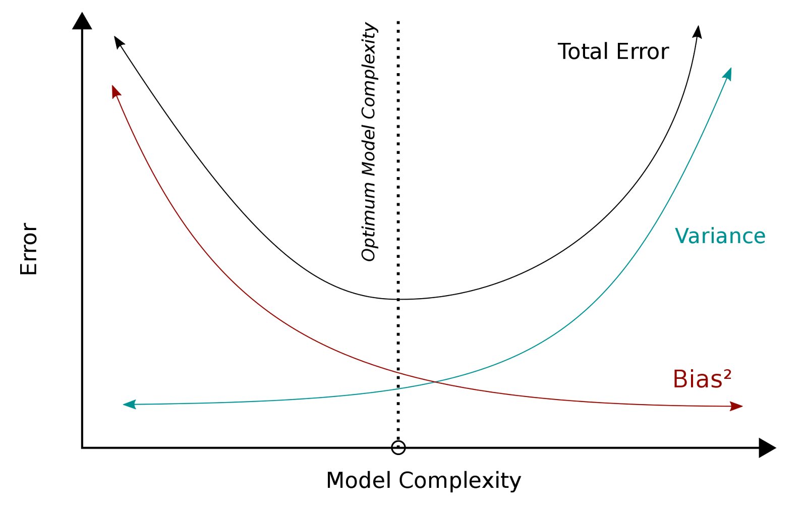
As model complexity increases, bias decreases but variance increases. The optimal balance minimizes total error.

5. Conclusion

  • Underfitting: High bias, low variance (too simple).
  • Overfitting: Low bias, high variance (too complex).
  • Optimal Model: Balances bias and variance for minimal generalization error.

Mathematical Derivation of Bias-Variance Tradeoff

1. Mathematical Setup

Let \( Y \) be the target variable and \( X \) be the predictor variable:

\[ Y = f(X) + e \]

  • \( e \) is the error term, normally distributed with \( \text{mean} = 0 \).
  • We build a model \( \hat{f}(X) \) to approximate \( f(X) \).

2. Expected Squared Error Decomposition

The expected squared error at a point \( x \) is:

\[ \text{Err}(x) = E\left[ (Y - \hat{f}(x))^2 \right] \]

This error can be decomposed into three components:

\[ \text{Err}(x) = \underbrace{\left( E[\hat{f}(x)] - f(x) \right)^2}_{\text{Bias}^2} + \underbrace{E\left[ (\hat{f}(x) - E[\hat{f}(x)])^2 \right]}_{\text{Variance}} + \underbrace{\sigma_e^2}_{\text{Irreducible Error}} \]

3. Components of Error

  • Bias²:
    • Measures the difference between the expected model prediction \( E[\hat{f}(x)] \) and the true value \( f(x) \).
    • Formula: \( \text{Bias} = E[\hat{f}(x)] - f(x) \).
  • Variance:
    • Measures the variability of model predictions around their mean.
    • Formula: \( \text{Variance} = E\left[ (\hat{f}(x) - E[\hat{f}(x)])^2 \right] \).
  • Irreducible Error:
    • Error caused by noise (\( \sigma_e^2 \)) in the data.
    • Cannot be reduced by improving the model.

4. Key Takeaways

  • Bias: High bias indicates underfitting (model oversimplifies the true relationship).
  • Variance: High variance indicates overfitting (model is too sensitive to noise).
  • Irreducible Error: Represents the inherent noise in the data.

Word Embedding Techniques

1. One Hot Encoding

One Hot Encoding converts categorical text data into numerical vectors. For a vocabulary of size \( N \), each word is represented as an \( N \)-dimensional vector where:

  • The index corresponding to the word is 1
  • All other indices are 0
Example: For vocabulary ["apple", "banana", "orange"], "banana" is encoded as [0, 1, 0].

2. TF-IDF (Term Frequency-Inverse Document Frequency)

TF-IDF quantifies the importance of a word in a document relative to a corpus. It combines:

Term Frequency (TF)

\[ \text{TF}(t, d) = \frac{\text{Number of times term } t \text{ appears in document } d}{\text{Total terms in } d} \] Example: For the document "He is Walter":

  • TF("He") = 1/3 ≈ 0.33
  • TF("Walter") = 1/3 ≈ 0.33

Inverse Document Frequency (IDF)

\[ \text{IDF}(t) = \log\left(\frac{\text{Total documents}}{\text{Documents containing } t}\right) \] Example (base 10 log):

  • For "He" (appears in all 3 documents): \(\log_{10}(3/3) = 0\)
  • For "is" (appears in 2 documents): \(\log_{10}(3/2) ≈ 0.176\)
  • For "Peter" (appears in 1 document): \(\log_{10}(3/1) ≈ 0.477\)

TF-IDF Calculation

\[ \text{TF-IDF}(t, d) = \text{TF}(t, d) \times \text{IDF}(t) \] Example with Smoothing (add 1 to avoid zeros):

Document 1 ("He is Walter"):
[1.0, 1.176, 1.477, 0.0, 0.0, 0.0, 0.0, 0.0]

Document 2 ("He is William"):
[1.0, 1.176, 0.0, 1.477, 0.0, 0.0, 0.0, 0.0]

Document 3 ("He isn’t Peter or September"):
[1.0, 0.0, 0.0, 0.0, 1.477, 1.477, 1.477, 1.477]

Key Differences

Technique Use Case Limitations
One Hot Encoding Simple categorical data High dimensionality for large vocabularies
TF-IDF Text classification, information retrieval Does not capture semantic meaning

Word2Vec: Word Embedding Technique

Introduction

Word2Vec is a neural network-based method for generating dense vector representations of words. Unlike sparse methods like One Hot Encoding, Word2Vec captures semantic and syntactic relationships between words by mapping them to vectors in a continuous vector space. Words with similar meanings or contexts are positioned closer together in this space.

Key Architectures

  • Continuous Bag of Words (CBOW):
    • Predicts a target word given its context words.
    • Faster training, suitable for smaller datasets.
    • Example: For the sentence "The cat sits on the mat", CBOW uses ["The", "cat", "on", "the", "mat"] to predict "sits".
  • Skip-Gram:
    • Predicts context words given a target word.
    • Better for rare words and large datasets.
    • Example: Uses "sits" to predict ["The", "cat", "on", "the", "mat"].

Mathematical Formulation

The objective is to maximize the log-likelihood of observing context words given a target word (Skip-Gram) or vice versa (CBOW). For Skip-Gram:

\[ \text{Maximize } \frac{1}{T} \sum_{t=1}^T \sum_{-c \leq j \leq c, j \neq 0} \log p(w_{t+j} | w_t) \]

Where:

  • \( T \): Total words in the corpus.
  • \( c \): Context window size.
  • \( p(w_{t+j} | w_t) \): Probability calculated using the softmax function: \[ p(w_O | w_I) = \frac{\exp(v_{w_O}^T v_{w_I})}{\sum_{w=1}^W \exp(v_w^T v_{w_I})} \]

Key Features

  • Dense Vectors: Typically 100-300 dimensions.
  • Semantic Relationships:
    • Analogies: \( \text{King} - \text{Man} + \text{Woman} ≈ \text{Queen} \).
    • Similar words: \( \text{Dog} ≈ \text{Puppy} \).
  • Efficiency: Uses techniques like Negative Sampling or Hierarchical Softmax to reduce computational cost.

Applications

  • Text classification
  • Named Entity Recognition (NER)
  • Machine translation
  • Recommendation systems

Advantages vs. Limitations

Advantages Limitations
Captures semantic relationships Fails to handle polysemy (e.g., "bank" as river vs. financial)
Low-dimensional embeddings Fixed context window size
Works well with small datasets Cannot handle out-of-vocabulary words

Conclusion

Word2Vec revolutionized NLP by enabling machines to understand word semantics through vector arithmetic. While newer models like BERT and GPT have emerged, Word2Vec remains foundational for tasks requiring lightweight, interpretable word embeddings.

Comparison of Word Embedding Techniques

Word Embedding Technique Main Characteristics Use Cases
TF-IDF
  • Statistical method to measure word relevance relative to a corpus.
  • Does not capture semantic relationships between words.
  • Information retrieval
  • Keyword extraction
Word2Vec
  • Neural network-based (CBOW and Skip-gram architectures).
  • Captures semantic and syntactic relationships between words.
  • Semantic analysis (e.g., word analogies like King - Man + Woman ≈ Queen)
  • Document similarity
GloVe
  • Uses matrix factorization based on global word-word co-occurrence statistics.
  • Addresses local context limitations of Word2Vec.
  • Word analogy tasks
  • Named-entity recognition (NER)
  • Comparable to Word2Vec in some tasks, superior in others.
BERT
  • Transformer-based architecture with attention mechanisms.
  • Captures bidirectional contextual information.
  • Language translation
  • Question-answering systems
  • Contextual search query understanding (e.g., Google Search)

Key Takeaways

  • TF-IDF: Best for simple relevance scoring without semantic understanding.
  • Word2Vec: Balances semantic understanding with computational efficiency.
  • GloVe: Enhances global context handling compared to Word2Vec.
  • BERT: State-of-the-art for tasks requiring deep contextual understanding.