Support Vector

Support Vector Machine (SVM) - Explained Simply

Support Vector Machine (SVM) is a supervised learning algorithm used for classification and regression tasks. However, it is mainly used for classification problems.

1. What is SVM?

SVM works by finding the best possible boundary (hyperplane) that separates data points of different classes. The goal is to maximize the margin between the classes while correctly classifying the data points.

• If the data is linearly separable, SVM finds a straight-line boundary (in 2D) or a hyperplane (in higher dimensions).
• If the data is not linearly separable, SVM uses the kernel trick to transform the data into a higher-dimensional space where it becomes separable.

2. Key Concepts in SVM

3. How SVM Works?

1. Find a hyperplane that best separates the classes.
2. Maximize the margin between classes.
3. Use support vectors to define the margin.
4. Classify new points based on their position relative to the hyperplane.

4. Types of SVM

A. Linear SVM

If the data is linearly separable, a straight hyperplane is used.

B. Non-Linear SVM (Kernel Trick)

If the data is not linearly separable, SVM uses kernel functions to map the data into a higher-dimensional space where a linear separator can be applied.

• Linear Kernel → For linearly separable data.
• Polynomial Kernel → For more complex boundaries.
• Radial Basis Function (RBF) Kernel → For highly non-linear data.
• Sigmoid Kernel → Similar to neural networks.

5. Mathematical Formulation

The equation of the hyperplane is:

w ⋅ x - b = 0

where:

• w = weight vector (normal to the hyperplane)
• x = feature vector
• b = bias term

For classification:

• If \( w \cdot x - b \geq 1 \) → Class 1
• If \( w \cdot x - b \leq -1 \) → Class -1

The optimization goal is: Maximize \( \frac{1}{\|w\|} \) subject to \( y_i (w \cdot x_i - b) \geq 1 \)

6. Advantages of SVM

• ✅ Effective for high-dimensional data
• ✅ Works well with small datasets
• ✅ Robust to outliers (with soft margin)
• ✅ Can handle non-linear problems using kernels

7. Disadvantages of SVM

• ❌ Computationally expensive for large datasets
• ❌ Choosing the right kernel can be tricky
• ❌ Less interpretable than simpler models

8. Applications of SVM

• 🔹 Image classification (e.g., face detection)
• 🔹 Text classification (e.g., spam detection)
• 🔹 Medical diagnosis (e.g., cancer detection)
• 🔹 Handwriting recognition

Conclusion

SVM is a powerful and versatile algorithm, especially for classification problems. Its ability to find the optimal decision boundary makes it a popular choice in machine learning.

Would you like a practical example or code implementation? 🚀

Support Vectors in SVM

In Support Vector Machine (SVM), support vectors are the data points closest to the decision boundary (hyperplane). These points are crucial because they determine the position and orientation of the hyperplane and influence the margin between classes.

Key Properties of Support Vectors

• They define the optimal hyperplane – Support vectors are the critical data points that affect the placement of the decision boundary.
• They lie closest to the hyperplane – The margin is calculated based on the distance of these support vectors from the hyperplane.
• They help maximize the margin – SVM creates a hyperplane with the maximum margin, ensuring the decision boundary is as far as possible from the support vectors.
• Only support vectors influence the decision boundary – Other data points that are farther away do not contribute to defining the hyperplane.

Support Vectors in SVM

In Support Vector Machine (SVM), support vectors are the data points closest to the decision boundary (hyperplane). These points are crucial because they determine the position and orientation of the hyperplane and influence the margin between classes.

Mathematical Representation

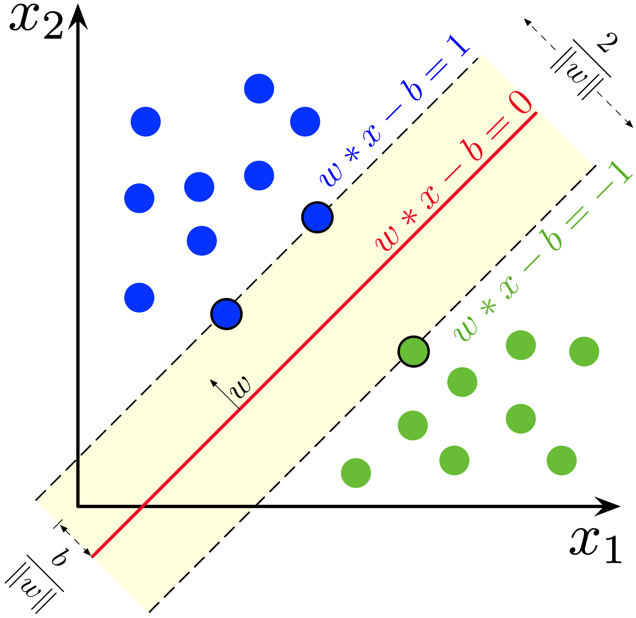
The decision boundary in SVM is represented as:

w · x - b = 0

where:

• w is the weight vector (defines the orientation of the hyperplane).
• x is the feature vector.
• b is the bias term.

The support vectors satisfy:

w · x_i - b = ±1

Visualization of Support Vectors

The diagram below represents the support vectors, the margin, and the decision boundary:

Key Properties of Support Vectors

• They define the optimal hyperplane – Support vectors are the critical data points that affect the placement of the decision boundary.
• They lie closest to the hyperplane – The margin is calculated based on the distance of these support vectors from the hyperplane.
• They help maximize the margin – SVM creates a hyperplane with the maximum margin, ensuring the decision boundary is as far as possible from the support vectors.
• Only support vectors influence the decision boundary – Other data points that are farther away do not contribute to defining the hyperplane.

Why Are Support Vectors Important?

• They make SVM robust – Even if non-support vector data points are removed, the model remains the same.
• They improve generalization – A well-defined margin ensures better performance on unseen data.
• They help in both linear and non-linear SVM – In non-linear SVM, a kernel function maps the data to a higher-dimensional space where it becomes linearly separable.

What do you mean by Hard Margin SVM?

In SVM, we try to find a hyperplane that maximizes the margin.

Assume three hyperplanes, namely \( \pi, \pi^+, \pi^- \), such that:

• \( \pi^+ \) is parallel to \( \pi \), passing through the support vectors on the positive side.
• \( \pi^- \) is parallel to \( \pi \), passing through the support vectors on the negative side.

Let this hyperplane be \( W^T X + b \), where \( W \) is perpendicular to the hyperplane.

For \( \pi^+ \): \( W^T X + b = 1 \) \( \Rightarrow W^T X + b - 1 = 0 \)
For \( \pi^- \): \( W^T X + b = -1 \) \( \Rightarrow W^T X + b + 1 = 0 \)

Margin Calculation:
\[ \text{Margin} = \frac{\text{difference of vector components} ||w||}{||W||} = \frac{(W^T X + b -1) - (W^T X + b+1)}{||W||} = \frac{| -2 |}{||W||} \]

Objective: Find \( (W^*, b^*) = \arg \max \frac{2}{||W||} \)

Constraints:

• \( y_i (W^T X + b) \geq 1 \) (For correctly classified points)
• \( y_i (W^T X + b) < 1 \) (For incorrectly classified points)

If the points are linearly separable, the hyperplane can distinguish them. However, if an outlier is introduced, the hyperplane may fail to separate them. This type of SVM is called a Hard Margin SVM because it has strict constraints to correctly classify each and every data point.

Kernel Function in SVM

A kernel function is a way of computing the dot product of two vectors \( x \) and \( y \) in some (possibly very high-dimensional) feature space. This is why kernel functions are sometimes called "generalized dot products."

The kernel trick is a method of using a linear classifier to solve a non-linear problem by transforming non-linear data into a higher-dimensional space where it becomes linearly separable.

Soft Margin SVM Formulation

As per the soft margin SVM formulation, the goal is to maximize the margin while allowing some misclassifications:

\[ w^*, b^* = \arg\max_{w, b} \frac{2}{\|w\|} = \arg\min_{w, b} \frac{\|w\|^2}{2} \]

The optimization problem with slack variables \( \zeta_i \) is:

\[ w^*, b^* = \arg\min_w \frac{\|w\|^2}{2} + C \sum_{i=1}^{n} \zeta_i, \] subject to \( y_i (w^T x_i + b) \geq 1 - \zeta_i \) for all points, where \( \zeta_i \geq 0 \).

Here, \( C \) is a hyperparameter that controls the trade-off between maximizing the margin and minimizing misclassification:

• High \( C \): Less tolerance for misclassification (overfitting risk).
• Low \( C \): More tolerance for misclassification (underfitting risk).

Dual Form of SVM Using Lagrange Multipliers

The alternative method is the dual form of SVM, which uses Lagrange multipliers to solve the constrained optimization problem:

\[ \max_{\alpha_i} \sum_{i=1}^{n} \alpha_i - \frac{1}{2} \sum_{i=1}^{n} \sum_{j=1}^{n} \alpha_i \alpha_j y_i y_j (x_i^T x_j) \]

Subject to:

• \( \alpha_i \geq 0 \)
• \( \sum_{i=1}^{n} \alpha_i y_i = 0 \)

- For every \( x_i \), there is a corresponding \( \alpha_i \). - \( x_i \) appears in the form of the dot product \( x_i^T x_j \). - \( x_i \) and \( x_j \) are data points from the training dataset. - Only points with \( \alpha_i > 0 \) are support vectors, while non-support vectors have \( \alpha_i = 0 \).

Kernel Trick & Similarity

Since the dual form depends only on the dot product \( x_i^T x_j \), we can replace it with a kernel function \( K(x_i, x_j) \) to enable SVMs to handle non-linearly separable data.

Some common kernel functions:

• Linear Kernel: \( K(x_i, x_j) = x_i^T x_j \)
• Polynomial Kernel: \( K(x_i, x_j) = (x_i^T x_j + c)^d \)
• Gaussian (RBF) Kernel: \( K(x_i, x_j) = e^{-\gamma \|x_i - x_j\|^2} \)

The kernel trick effectively transforms the data into a higher-dimensional space where it becomes linearly separable, without explicitly computing the transformation.

Why is SVM Called a Maximum Margin Classifier?

Suppose we are given a dataset containing two classes and asked to build a classifier. This dataset can be perfectly separated using a hyperplane. However, there are infinitely many such separating hyperplanes. We need a reasonable way to decide which hyperplane to use as a classifier.

Support Vector Machine (SVM) is a type of classifier that finds the optimal hyperplane that best separates the positive and negative classes. The key idea behind SVM is to maximize the margin between the two classes while maintaining classification accuracy.

What is the Maximum Margin?

The margin is the distance between the separating hyperplane and the closest data points from either class (these closest points are called support vectors).

The optimal hyperplane is the one that maximizes this margin, ensuring the classifier is:

• Less sensitive to small variations in data (reducing overfitting).
• More generalizable to unseen data.
• Equidistant from both classes, providing a balanced decision boundary.

Mathematical Formulation

Given a dataset \( (x_i, y_i) \) where \( y_i \in \{-1, 1\} \), the decision boundary is defined by:

\[ w \cdot x + b = 0 \]

The margin is defined as:

\[ \frac{2}{\|w\|} \]

To find the optimal hyperplane, we solve the following optimization problem:

\[ \min_{w, b} \frac{\|w\|^2}{2} \] Subject to: \[ y_i (w \cdot x_i + b) \geq 1, \quad \forall i \]

This ensures that the margin is maximized while correctly classifying all data points.

Conclusion

Since SVM explicitly aims to maximize the margin while maintaining correct classification, it is called a Maximum Margin Classifier.

Is SVM Affected by Outliers?

Yes, Support Vector Machine (SVM) is affected by outliers, but its impact depends on the type of SVM used.

1. Hard Margin SVM (Strict Separation)

• In Hard Margin SVM, we assume that data is perfectly separable, meaning no misclassification is allowed.
• Problem: A single outlier can drastically change the position of the decision boundary, making the model highly sensitive to noise.

🚫 Hard Margin SVM is highly affected by outliers.

2. Soft Margin SVM (Allows Some Misclassification)

• Soft Margin SVM introduces a slack variable \( \zeta_i \) to allow some points to be misclassified.
• This helps in handling outliers by introducing a trade-off between maximizing the margin and minimizing misclassification.

✅ Soft Margin SVM is less affected by outliers compared to Hard Margin SVM.

3. Kernel SVM (Non-Linear Decision Boundary)

• If an outlier is too far from the majority of data points, a kernel function (e.g., RBF, polynomial) can help by mapping data to a higher-dimensional space.
• However, if outliers are within the decision boundary, they may still influence the hyperplane.

⚖ Effect of outliers depends on the kernel and regularization parameters.

How to Reduce the Effect of Outliers in SVM?

• Use Soft Margin SVM: Allows some flexibility to handle outliers.
• Tune the Regularization Parameter (C):
  • A lower C value allows more misclassifications, reducing sensitivity to outliers.
  • A higher C enforces strict classification, making it more sensitive to outliers.
• Use Robust Kernel Functions: RBF and polynomial kernels can help in non-linearly separable data.
• Preprocess Data:
  • Detect and remove extreme outliers using techniques like IQR (Interquartile Range) or Z-score.
  • Normalize/scale features to reduce the impact of large values.

Conclusion

• Hard Margin SVM is highly sensitive to outliers.
• Soft Margin SVM handles outliers better by allowing some misclassification.
• Proper tuning of hyperparameters and data preprocessing can minimize outlier effects.

Relation Between KNN and Kernel SVM

1. Understanding KNN and Kernel SVM

• K-Nearest Neighbors (KNN): A non-parametric, instance-based learning algorithm that classifies a point based on the majority class of its k-nearest neighbors.
• Kernel SVM: A model that maps data to a higher-dimensional space using a kernel function, allowing it to find non-linear decision boundaries.

2. Key Similarities

• Both work well with non-linearly separable data: KNN uses local decision boundaries, while Kernel SVM transforms data using kernels.
• Both rely on similarity:
  • KNN classifies based on distance (e.g., Euclidean, cosine similarity).
  • Kernel SVM uses a kernel function (e.g., RBF, polynomial) to compute similarity.
• Both can approximate each other:
  • A well-tuned **Kernel SVM with RBF kernel** can behave like a smoothed version of KNN.
  • KNN with **proper k selection** can approximate the decision boundary of a Kernel SVM.

3. Differences Between KNN and Kernel SVM

Aspect	KNN	Kernel SVM
Type	Instance-based (Lazy learning)	Model-based (Optimized decision boundary)
Computational Cost	High at test time (O(n))	High at training time (O(n²) or more)
Decision Boundary	Flexible but noisy for small k	Smooth and well-regularized
Handling High-Dimensional Data	Struggles with high dimensions (curse of dimensionality)	Performs well with appropriate kernels
Outlier Sensitivity	Highly affected	Can be tuned using soft margin

4. When to Use KNN vs. Kernel SVM

• Use KNN when:
  • The dataset is small and low-dimensional.
  • A simple, interpretable model is needed.
  • Real-time learning is not required.
• Use Kernel SVM when:
  • The dataset has complex, non-linear relationships.
  • High accuracy is required with a well-defined decision boundary.
  • There is enough computational power for training.

5. Connection Between KNN and Kernel SVM

Kernel SVM can be seen as a more sophisticated and optimized version of KNN, where instead of directly using distances, we transform the space using kernels to define better decision boundaries.

In fact, some research suggests that Kernel SVM with an RBF kernel behaves similarly to KNN but in a more controlled manner by learning an optimal distance metric rather than relying on raw Euclidean distances.

Conclusion

• Both KNN and Kernel SVM rely on similarity and can approximate each other under certain conditions.
• KNN is simpler but computationally expensive at test time, whereas Kernel SVM is computationally heavy at training time but efficient at prediction.
• Choosing between them depends on dataset size, dimensionality, and computational constraints.

Hyperparameters in Stochastic Gradient Descent (SGD) with Hinge Loss

1. Understanding SGD with Hinge Loss

Stochastic Gradient Descent (SGD) is an optimization algorithm used for training machine learning models, especially in linear classifiers like SVM (Support Vector Machine). Hinge Loss is the loss function used in SVM, which penalizes misclassified points.

2. Key Hyperparameters in SGD with Hinge Loss

• Learning Rate (η): Determines the step size for updating weights. A small η leads to slow convergence, while a large η may cause instability.
• Regularization Parameter (λ): Controls the trade-off between margin maximization and classification error. Helps prevent overfitting.
• Batch Size: Defines how many training samples are used to compute gradients before updating weights.
• Number of Epochs: The number of times the algorithm processes the entire dataset.
• Decay Rate: Reduces the learning rate over time to fine-tune convergence.
• Momentum: Helps accelerate learning by maintaining a moving average of past gradients.

3. Hinge Loss in Support Vector Machine (SVM)

Hinge loss is defined as:

\( L(y, f(x)) = \max(0, 1 - y f(x)) \)

where:

• \( y \) is the actual label (-1 or +1).
• \( f(x) \) is the predicted score from the model.
• The loss is 0 if the sample is correctly classified and lies beyond the margin.

4. Graphical Representation of Hinge Loss

Below is a diagram illustrating hinge loss:

Key Observations:

• If the prediction is correct and far from the decision boundary, the loss is 0.
• If the point is close to the boundary but correctly classified, the loss is small.
• If the point is misclassified, the loss increases linearly.

5. Why Use Hinge Loss?

• Encourages a larger margin between classes, improving generalization.
• Helps deal with outliers by penalizing only those that fall within the margin.
• Works well in scenarios where class separation is important, such as text classification and image recognition.

Conclusion

SGD with hinge loss is commonly used in SVM and linear classifiers. The choice of hyperparameters, such as learning rate and regularization, plays a crucial role in model performance. Hinge loss helps in maximizing the margin and improving classification robustness.

Kernel SVM vs. Linear SVM (SGD Classifier with Hinge Loss) - Latency Comparison

1. Difference Between Kernel SVM and Linear SVM (SGD Classifier)

• Kernel SVM: Uses different kernels (e.g., RBF, polynomial) to transform data into a higher-dimensional space, allowing it to handle non-linearly separable data.
• Linear SVM (SGD Classifier with Hinge Loss): Uses stochastic gradient descent (SGD) with hinge loss to optimize a linear decision boundary.

2. Latency Comparison

Kernel SVM is computationally expensive because:

• It computes a kernel function for every pair of data points, leading to a complexity of \( O(n^2) \) or worse.
• Training requires solving a quadratic optimization problem, which is slow for large datasets.

SGD Classifier with Hinge Loss has lower latency because:

• It approximates SVM using online learning, processing one batch at a time.
• Its training complexity is roughly \( O(n) \), making it scalable for large datasets.
• It is suitable for linear problems but does not work well for complex non-linear decision boundaries.

3. When to Use Each?

• Use SGD Classifier with Hinge Loss when the data is linearly separable or approximately linear.
• Use Kernel SVM when the data has complex decision boundaries and requires transformations for better separation.
• If using an RBF kernel, SGD is not suitable since it only optimizes linear models.

Conclusion

SGD Classifier with Hinge Loss is preferred for large-scale, linear problems due to its lower latency, while Kernel SVM is better for non-linear problems but is computationally expensive.

Computing Feature Importance in SVM

1. Feature Importance in Linear SVM

For an SVM classifier with a linear kernel, feature importance can be determined using the weight vector \( w \):

• The decision function for linear SVM is \( f(x) = w \cdot x + b \).
• The magnitude of each component of \( w \) represents the importance of the corresponding feature.
• Feature importance can be ranked using \( |w_i| \), where larger values indicate more influential features.

2. Feature Selection in SVM

Feature selection techniques like Forward Feature Selection can be used to identify important features iteratively:

• Start with an empty set of features.
• Add features one by one and train the SVM model.
• Keep the feature that improves classification performance the most.
• Repeat until performance stops improving.

3. Why Feature Importance is Difficult in Non-Linear SVM

For SVM with non-linear kernels (e.g., RBF, polynomial):

• The kernel function transforms data into a higher-dimensional space.
• Feature importance is not directly related to the original input space.
• Unlike linear SVM, there is no explicit weight vector \( w \) for feature importance computation.

4. Alternative Methods for Non-Linear SVM

Although feature importance is not directly available for non-linear SVM, alternative methods include:

• PCA (Principal Component Analysis): Identifies dominant patterns in the transformed space.
• Permutation Feature Importance: Measures change in model accuracy when shuffling feature values.
• SHAP (SHapley Additive Explanations): Provides feature importance scores based on model predictions.

Conclusion

Feature importance in SVM is straightforward for a linear kernel (using weights \( w \)), but for non-linear kernels, indirect methods like PCA, permutation importance, or SHAP are required.

Alpha Value for Non-Support Vectors

In Support Vector Machines (SVM), the alpha values (\(\alpha_i\)) are the Lagrange multipliers that determine the contribution of each data point to the decision boundary.

Key Points:

• For support vectors: \( \alpha_i > 0 \), meaning they actively contribute to the decision boundary.
• For non-support vectors: \( \alpha_i = 0 \), meaning they do not influence the final classifier.

Mathematical Explanation:

In the dual formulation of SVM optimization:

\( L(\alpha) = \sum_{i=1}^{n} \alpha_i - \frac{1}{2} \sum_{i=1}^{n} \sum_{j=1}^{n} \alpha_i \alpha_j y_i y_j K(x_i, x_j) \)

Subject to:

\( \sum_{i=1}^{n} \alpha_i y_i = 0, \quad 0 \leq \alpha_i \leq C \)

Conclusion:

Only the support vectors have nonzero \(\alpha_i\), while non-support vectors have \(\alpha_i = 0\), meaning they do not contribute to the final decision function.

Training and Runtime Complexities of SVM

Training Complexity

• SVM training can be performed using Stochastic Gradient Descent (SGD) for linear SVM.
• For kernel SVMs, a specialized algorithm like Sequential Minimal Optimization (SMO) is used.
• Example: libSVM is a widely used library for training SVMs.
• Training Time Complexity: \( O(n^2) \) for kernel SVMs.
• Since training complexity is quadratic in the number of samples \( n \), SVMs are not preferred for very large datasets.

Runtime Complexity

• Run Time Complexity: \( O(kd) \), where:
  • \( k \) is the number of support vectors.
  • \( d \) is the dimensionality of the input space.
• Since the prediction time depends on the number of support vectors, SVMs with a large number of support vectors may have higher inference time.

Special Cases of SVM

Feature Engineering

• Kernelization can be applied to map data into higher-dimensional space.

Decision Surfaces

• SVM can learn non-linear decision surfaces using kernel functions.

Similarity or Distance Function

• SVM models can use custom kernel functions to measure similarity or distance effectively.

Interpretability and Feature Importance

• For a linear kernel classifier, feature importance can be found using forward feature selection.
• For other kernels, feature importance is not directly interpretable since data is transformed into a new space.

Impact of Outliers

• Support Vectors determine the decision boundary, so outliers typically have little impact.
• However, for RBF kernels with a small sigma, outliers may affect the decision boundary, similar to k-NN with small \( k \).

Bias-Variance Tradeoff

• High C (Regularization Parameter): Leads to overfitting, resulting in high variance.
• Low C: Causes underfitting, resulting in high bias.

Handling Large Dimensionality

• SVM performs well in high-dimensional spaces (large \( d \)).
• However, when the dataset size or the number of support vectors is very large, SVMs can become computationally expensive.
• In such cases, Logistic Regression is often preferred.

Various Kernels in SVM

Kernels are mathematical functions that transform data into higher dimensions to make it linearly separable. The choice of the kernel function significantly affects the performance of an SVM model.

1. Linear Kernel

The simplest kernel, used when data is already linearly separable.

Formula: \( K(x, y) = x \cdot y \)

• Computationally efficient.
• Works well with high-dimensional sparse data (e.g., text classification).
• Not suitable for non-linearly separable data.

2. Polynomial Kernel

Maps input features into a higher-dimensional space using polynomial transformation.

Formula: \( K(x, y) = (x \cdot y + c)^d \), where \( d \) is the degree of the polynomial.

• Good for capturing feature interactions.
• Computationally expensive for high-degree polynomials.

3. Radial Basis Function (RBF) Kernel

The most commonly used kernel. It maps data into an infinite-dimensional space.

Formula: \( K(x, y) = \exp(-\gamma ||x - y||^2) \)

• Works well with complex decision boundaries.
• \( \gamma \) controls how much influence a single training example has.
• Can overfit if \( \gamma \) is too large.

4. Sigmoid Kernel

Inspired by neural networks, it behaves like an activation function.

Formula: \( K(x, y) = \tanh(\alpha x \cdot y + c) \)

• Less commonly used compared to RBF.
• Can behave inconsistently with different values of \( \alpha \) and \( c \).

5. Custom Kernels

Custom similarity functions can be designed based on domain knowledge.

• Can be useful for specialized tasks.
• Needs to satisfy Mercer’s theorem (must be a valid positive semi-definite function).